Tuesday, September 16, 2014

ETF Investment System (16 Assets)

Explanation of ETF Investment System covering 5 major assets is at the following link: "A Minimum Variance ETF Investment System".

Explanation of ETF Investment System covering 10 assets is at the following link: "ETF Investment System (10 Assets)".

If expanding investing pool to 16 of the most actively traded ETFs in the U.S., and allocate equal capital to the two ETFs with the highest values of the "Investment Value Index". The equity growth curve of the new ETF Investment System model from January 2003 to September 2014 is as follows: 


This new aggressive investment system increases annual percentage return dramatically comparing to the previous two conservative models (+14.5% and +18.4% vs. +43.8%). Two factors affect the result. First,  there are a few very volatile funds in the 16 of the most actively traded ETFs (such as Brazil and China ETF funds). Long-term investment returns turn to have positive correlation with volatility. Second and more importantly, trading signals of the new investment system are generated one week earlier than previous models (forward-looking one week). The difference between early and late signals are illustrated in the following charts:

Investment model with early signals (1 out of 16 ETFs)


Investment model with late signals (1 out of 16 ETFs)


Therefore, we will follow the new more aggressive ETF Investment System (16 Assets) from now on to replicate its equity growth curve.


======

http://murmurhudson.com 


Saturday, August 23, 2014

ETF Investment System (10 Assets)

Explanation of ETF Investment System covering 5 assets is at the following link: "A Minimum Variance ETF Investment System"

If in addition to the 5 major asset classes (cash, long-term Treasury bonds, gold, U.S. large-cap stocks, and real estate), add another 5 stock indices: U.S. small-cap stock index, European stock index, Japan stock index, Asia-Pacific emerging market stock index, and Latin-America stock index. 


Again, allocate equal capital to the two ETFs with the highest values of the "Investment Value Index". The equity growth curve of the new ETF Investment System model from January 2003 to August 2014 is as follows:


With small increase of volatility, ETF Investment System Of 10 Assets enhances annual return percentage from +14.5% to +18.4% (equity increased to 7 times in 11.5 years). Therefore, the advantage of the new ETF Investment System is obvious.


======

http://murmurhudson.com

Monday, September 23, 2013

A Minimum Variance ETF Investment System

At any moment when market opens, a software program that I designed calculates the value of the proprietary "Investment Value Index" for each of the following five major asset classes represented by their respective ETFs: cash (SHY), long-term Treasury bonds (TLT), gold (GLD), stocks (SPY), and real estate (IYR). Then, I allocate equal capital to the two ETFs with the highest values of the "Investment Value Index".

For example, suppose on February 1st, 2012, the two assets with the highest value of the "Investment Value Index" were cash and long-term Treasury bonds, I would allocate equal amount of capital to SHY and TLT. If on February 2nd, 2012, the two assets with the highest value of the "Investment Value Index" changed to gold and long-term Treasury bonds, I would exchange SHY to GLD, and continue to hold TLT.
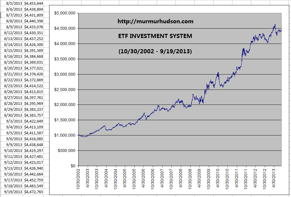
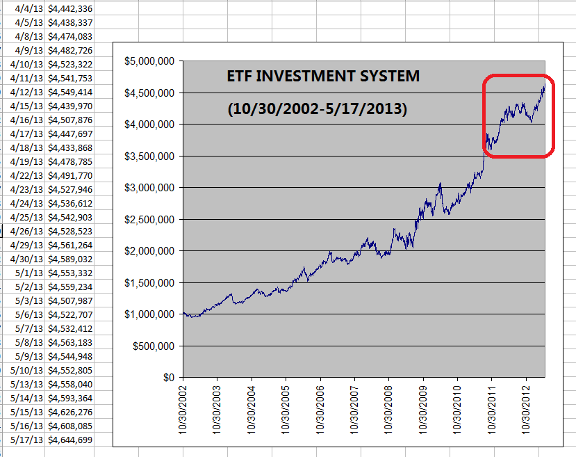
The following chart is the equity growth curve of the ETF Investment System model from 10/30/2002 to 9/19/2013:
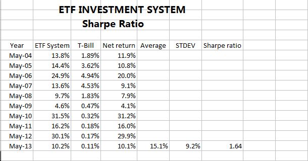

The following is the Sharpe ratio calculation of the ETF Investment System (Sharpe ratio 1.4 from January 2004 to September 2013):


Additional improvement on this very simple yet elegant investment system is as follows.

Suppose ETF Investment System holds TLT and SPY, each with 50% of total investing capital. But the volatility of SPY is substantially higher than that of TLT. If each ETF has the same amount of capital, SPY would contribute more than TLT in term of both upside and downside. To account for this, volatility adjustment is needed to balance risk.

Suppose again, ETF Investment System holds SPY and IYR, each with 50% of total investing capital. But there may be a strong positive correlation of price movement between SPY and IYR. If each ETF has the same amount if capital, the SPY and IYR portfolio would have much higher volatility than the SPY and GLD portfolio, which may have negative correlation of price movement between the two. In this case, correlation adjustment is needed to minimize risk.
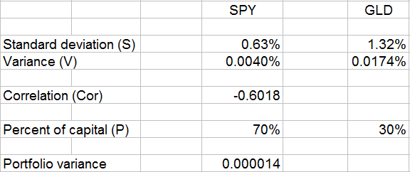
The calculation to construct a minimum variance portfolio is shown below.


In this hypothetical example, SPY and GLD have a negative correlation of –0.6018 and volatility of GLD is more than double that of SPY. Therefore, allocation of capital should be 70% SPY and 30% GLD to achieve minimum variance.

Indeed, portfolio variance is a very low number of 0.000014.

Equity growth curve of the minimum variance ETF Investment System portfolio is shown below (from 10/30/2002 to 10/11/2013).


Annualized return: +15.5% compare to +14.1% before)

Maximum drawdown: -13.8% (compare to –15.9% before)

Sharpe ratio: 1.4 (same as before 1.4)

The following is the Sharpe ratio calculation of the minimum variance ETF Investment System (Sharpe ratio 1.4 from January 2003 to October 2013).


The minimum variance ETF Investment System improves the original system significantly in term of risk reduction. Historical maximum drawdown is reduced from –15.9% to –13.8%. Average annual return in the past 11 years is also enhanced from +14.1% to +15.5%. Initial investment capital is increased to almost 5-fold. Sharpe ratio is maintained at 1.4 as before.

Higher return with much reduced volatility, the minimum variance ETF Investment System proves to be a worthwhile modification of the original ETF Investment System.

In some retirement accounts and pension plans, participants can only invest in 3 of the 5 major assets: cash, long-term Treasury bonds, and stocks. Therefore, I have modified the ETF Investment System with these three asset classes.

At any moment when market opens, a software program that I designed calculates the value of the proprietary "Investment Value Index" for each of the following 3 major asset classes: cash, long-term Treasury bonds, and stocks. Then I allocate 100% of the capital to the ETF or mutual fund with the highest value of the "Investment Value Index".

For example, suppose on February 1st, 2012, the asset with the highest value of the "Investment Value Index" was cash, I would allocate 100% of the capital to a money market mutual fund. If on February 2nd, 2012, the asset with the highest value of the "Investment Value Index" changed to long-term Treasury bonds, I would exchange the money market mutual fund to a mutual fund holding long-term Treasury bonds.
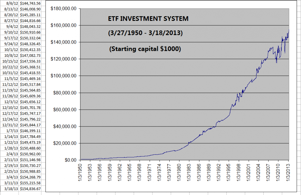

To evaluate the long-term effectiveness of the ETF Investment System, I back-tested with historical data from March 1950 to March 2013 for the following three asset classes: 3-month Treasury Bills (representing cash), 10-year Treasury bonds (representing long-term bonds), and S&P 500 Index (representing stocks). 

The following chart is the equity growth curve of the ETF Investment System model from March 1950 to March 2013 (starting with $1000 initial capital):


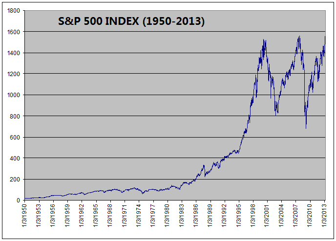
For comparison, this is the price chart for S&P 500 Index from March 1950 to March 2013:


 In the past 63 years, ETF Investment System increased the initial capital 155 times (from $1,000 to $154,836). Meanwhile, the return for S&P 500 Index was 90 times (from 17.29 to 1556.89).
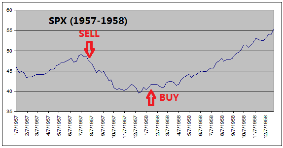
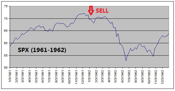
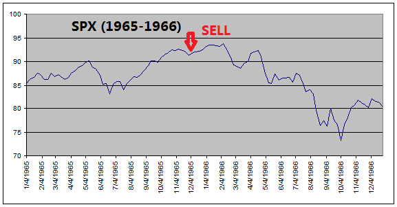
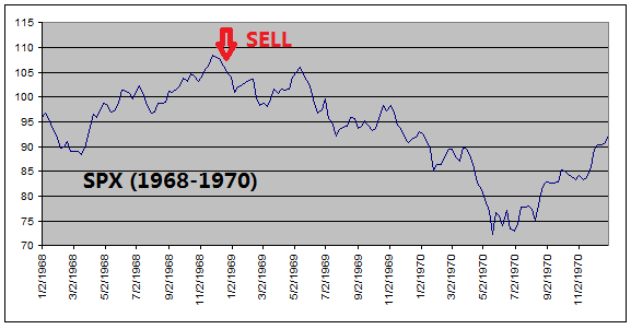
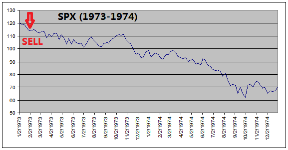
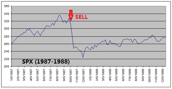
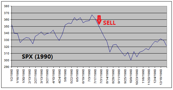
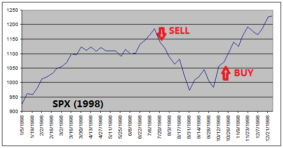
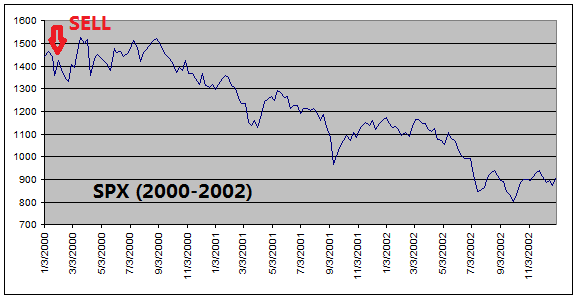
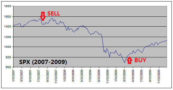
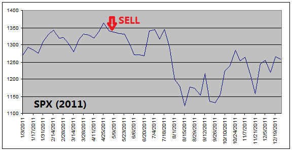

The reason that ETF Investment System outperforms the equity index is because it got out of equities before every major stock market downturns (see charts below).


In summary, ETF Investment System is a 100% quantitative and mechanical investment system. It holds only 2 of the 5 ETFs of major asset classes at any time (or holds 1 of the 3 ETFs with the ETF Investment System for retirement accounts). It is simple, easy to follow, and trades about 25 times per year. Above all, it fulfills the ultimate winning investment principle of "cut losses short, let profits run".


Disclosure: I hold 2 of the following 5 ETFs in my real brokerage account: SHY, TLT, GLD, SPY, and IYR.

======

http://murmurhudson.com

Friday, May 24, 2013

Sharpe Ratio of ETF Investment System

Sharpe ratio = Average investment return in excess of risk-free rate / Standard deviation of net investment returns

Sharpe Ratio of ETF Investment System is 1.64. 

Detailed calculation is shown below:

 
========

Murmur Hudson Investments website: 


http://murmurhudson.com


Sunday, April 14, 2013

Saturday, March 23, 2013

ETF Investment System Outperforms In Bear Market

In ETF Investment System Since 1950, I compared the performance of the ETF Investment System with S&P 500 index:


Why can ETF Investment System outperform the S&P 500 index? The reason is that ETF Investment System got out of stocks before every stock market corrections. 


Now, the U.S. stock market is close to a new high again. But history shows that stock market will eventually fall deeply every few years. And ETF Investment System shines more brightly in every bear market. I look forward to the performance of my real investment account in the next downturn. 


========

Murmur Hudson Investments website: 


http://murmurhudson.com


Sunday, March 17, 2013

Evidences That ETF System Works

In "ETF Investment System 2.0", I've shown the equity growth curve of the ETF Investment System for the last 10 years:


Will this model work in real live trading? There are several ways to prove it. 

One method is to open a real account and see if it actually follows the ETF model. This is exactly what I did. I opened an account at Scottrade in October 2012 with $100,000 of my own capital and started following the ETF Investment System. 


This first chart shows the equity curve of the ETF model from 1/3/2012 to 4/26/2013 (also shown in the red section of the above chart):


This second chart shows the equity curve of my investment account at Scottrade in the last 6 months (Daily equities in dollar amount are recorded publicly in my Blog at http://blog.wenxuecity.com/myindex/48731/.) :


As one can see clearly, the two charts look quite similar to each other. Although five months of data is short, it proves the point that the ETF model can be replicated in real investment situations. I will keep following ETF Investment System with this account and update results regularly.

Another method to show that the ETF model works is to apply the principal of the ETF System to a different set of investment vehicles and see if it would generates similar results. Instead of using ETFs of five major asset classes (SHY, TLT, GLD, SPY, and IYR), this time I apply the principal of the ETF System to currency trading, using US Dollar, Euro, Japanese Yen, and British pound as investment vehicles.


The following is the equity curve of ETF Investment System in currency trading in the past 5 years (without leverage):


As one can see clearly, the upward trend of this chart looks quite similar to that of the original ETF Investment System shown above.


In summary, the ETF Investment System is a 100% quantitative and mechanical investment system. It is simple, easy to follow, and trades not very often. It can be applied to not only the five major asset classes, but also in currency trading. More importantly, it works in the real world.


========


Murmur Hudson Investments website: 


http://murmurhudson.com